↜ Back to index Introduction to Numerical Analysis 1
Part a—Lecture 4
In this lecture we discuss simple generalizations of the Euler method. Report 1 is assigned below. Submit it to Acanthus portal LMS by May 10.
Higher order numerical methods for ODEs
We discussed the Euler method for the first order ODE \left\{ \begin{aligned} y' &= f(t, y), \qquad t > 0,\\ y(0) &= y_0. \end{aligned} \right.
The Euler method has error proportional to the step size h. This means that if we halve the step size (that is, do twice as many steps), we get a solution with half the error. This is why the Euler method is a first-order method (error proportional to h^1). Can we do better? 🤔
Yes, we can. For instance, we can use the midpoint method:
\begin{aligned} \text{For each $n = 0, 1, \ldots$ do}&\\ k_n &= y_n + \tfrac h2f(nh, y_n)\\ y_{n+1} &= y_n + h f\Big((n + \tfrac 12) h, k_n\Big) \end{aligned}
The idea is to do an extra step with the Euler method which gives k_n, an approximate value of the solution at the midpoint of the interval (nh, (n+1)h), and then use the value of f at this midpoint for the actual update. This way we get a much more accurate approximation of the integral of the right-hand side f(t,y(t)) over the interval (nh, (n+1)h).
For each step we have to do twice as much work than for the usual Euler method. But the midpoint method has error proportional to the square of the step size (h^2). Therefore it is a second-order method. In other words, if we halve the step size, we get four times smaller error. This is a huge difference. If we need to decrease the error 1 millon times, we need to take only 1000 times more steps, not 1 millon times more steps as in the Euler method.
In practice, 4th-order Runge-Kutta method is very popular (error proportional to h^4). But even higher order methods are used in more advanced solvers.
Backward Euler method
In Lecture 3, Exercise 2 we saw that for y' = -100y the Euler method had strange oscillations and the numerical solution was even blowing up when the step size was larger than 1/50.
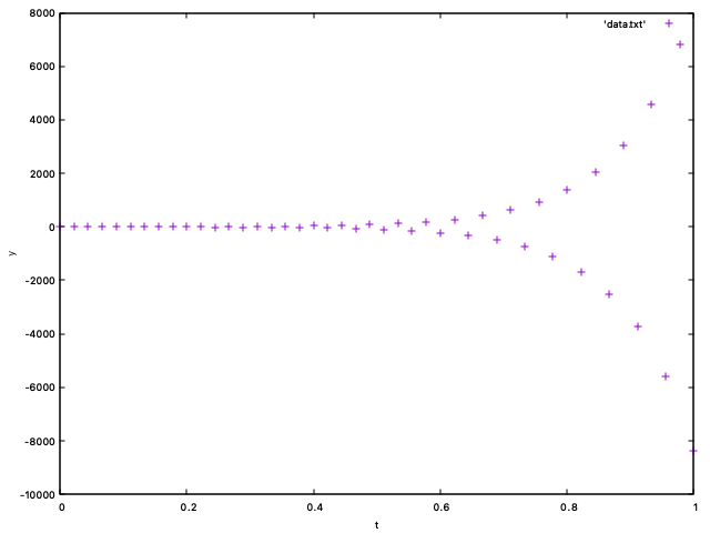
Let us try to understand this. One step of the Euler method for this ODE is y_{n+1} = y_n - 100 h y_n = (1 - 100 h) y_n. Clearly if h \geq 1/50 we have 1 - 100 h \leq -1 and therefore y_n cannot converge to 0, even though the exact solution of y' = -100 y is y(t) = y_0 e^{-100 t}.
An ODE where the time step h must be taken very small than would be expected from the error estimate to get a reasonable solution is referred to as stiff (硬い方程式).
For such ODEs we can use an implicit method, for example the backward Euler method:
y_{n+1} = y_n + hf\big(t_{n+1}, y_{n+1}\big), where t_{n+1} = (n+ 1)h. The difference from the usual (forward) Euler method is where the function f is evaluated: we evaluate it at the new point (t_{n+1}, y_{n+1}), not the old point (t_n, y_n).
We derived the forward Euler method by using the Taylor expansion of y at t = 0. The backward Euler method is derived by considering the Taylor expansion at t = h: y(0) = y(h) - h y'(h) + \tfrac 12 h^2 y''(\theta) \qquad \text{for some } \theta \in (0, h). We therefore also expect that the numerical error at each step is proportional to h^2, and after n steps it is proportional to h^1: it is a first-order method.
The disadvantage of using this method is that to find y_{n+1}, we must in general solve a nonlinear equation y_{n+1} - hf\big(t_{n+1}, y_{n+1}\big) = y_n for y_{n+1}. This makes backward Euler method more difficult to use.
Example 1. Let us apply the backward Euler method to y' = -100 y with y_0 = 1. The formula is y_{n+1} - h (-100 y_{n+1}) = y_n, from which y_{n+1} = \frac{y_n}{1 + 100h}. We get a solution y_n = \frac{y_0}{(1 + 100 h)^n}. Note that this converges to 0 monotonically for any h > 0 and we do not have any issues with oscillations or instability as in the case of the forward Euler method.
Systems of ODEs
We can easily generalize all the discussed numerical methods to systems of ordinary differential equations like
\begin{aligned} y_1'(t) &= f_1(t, y_1(t), y_2(t))\\ y_2'(t) &= f_2(t, y_1(t), y_2(t))\\ \end{aligned} where f_1, f_2 are given functions. We need an initial condition for each equation y_1(0) = y_{0,1}, \qquad y_2(0) = y_{0,2}.
Example 2. A simple example is the system \begin{aligned} y_1' &= y_2\\ y_2' &= -y_1 \end{aligned} which describes a harmonic oscillator (調和振動子) with y_1(t) the position and y_2(t) the velocity.
The solution is \begin{aligned} y_1(t) &= y_{0,1} \cos t + y_{0,2} \sin t\\ y_2(t) &= -y_{0,1} \sin t + y_{0,2} \cos t \end{aligned}
In general, for N \in {\mathbb{N}} we consider f(t, y) = (f_1(t, y), f_2(t, y), \ldots, f_N(t, y)) a vector valued function and y(t) = (y_1(t), y_2(t), \ldots, y_N(t)) a vector valued solution of the ODE system \left\{ \begin{aligned} y'(t) &= f(t, y), \qquad t > 0, \\ y(0) &= y_0, \end{aligned} \right. where y'(t) = (y_1'(t), y_2'(t), \ldots, y_N'(t)) and y_0 = (y_{0,1}, y_{0,2}, \ldots, y_{0, N}) is a given initial data.
The numerical methods can be easily extended to solve a system by simply considering y_n in the formula to be a vector: y_n = (y_{n, 1}, y_{n, 2}, \ldots, y_{n, N}).
Here is an implementation of the Euler method for the system in y_1' = y_2, y_2' = - y_1 in Fortran.
! Implementation of the Euler method for a system y_1' = y_2, y_2' = - y_1
implicit none
integer i, n
real y1, y2, y1new, y2new, h, t

n = 100
h = 10. / n

! Initial data
y1 = 1.
y2 = 0.
print *, 0., y1, y2

do i = 1, n
    !👇 we cannot update y1 yet since we need it for y2
    y1new = y1 + h * y2
    !                👇 here we need the old value of y1
    y2new = y2 - h * y1

    y1 = y1new
    y2 = y2new

    print *, i * h, y1, y2
enddo

end
Alternatively, it is convenient to use arrays to store y.
! Implementation of the Euler method for a system y_1' = y_2, y_2' = - y_1
implicit none
integer i, n
real h, t
! declare y as an array of 2 reals referred to as y(1) and y(2)
real y(2)

n = 100
!   👇 solve on interval (0, 10)
h = 10. / n

! Initial data
y = [1., 0.]
print *, 0., y

do i = 1, n
    ! array operations are performed element-wise
    y = y + h * [y(2), -y(1)]
                  ! 👇 prints all values in the array
    print *, i * h, y
enddo

end- Note that we do not need to store the old value of y_1 and y_2 when using arrays since the right-hand side of
y = y + h * [y(2), -y(1)]is computed first using the old values before they are overwritten.
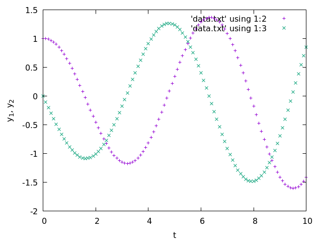
Here is a plot of the numerical solution.
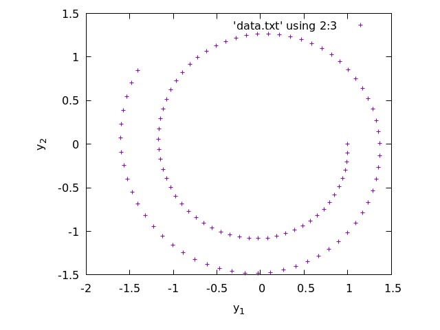
And here is a parametric plot of the solution. The points represent (y_{1,i}, y_{2,i}) for i = 0, \ldots, n.
To produce these plots, the numerical solution was stored in a file using
./a.exe > data.txtThen I plotted them using the following gnuplot commands:
first plot
set xlabel 't'
set ylabel 'y_1, y_2'
plot 'data.txt' using 1:2, 'data.txt' using 1:3
second plot
set size ratio -1
set xlabel 'y_1'
set ylabel 'y_2'
plot 'data.txt' using 2:3
set size ratio -1is used to set the same units on both axes.
Note that the Euler method produces a solution that looks like a spiral, while the plot of the actual solution is a circle.
Report 1
Submit the solutions of the 4 problems to Acanthus portal. Each subproblem is worth 10 points.
As the title of each plot, use your full 10-digit student number: set title '0123456789'.
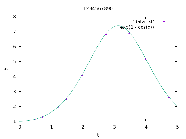
Exercise 1. Implement the midpoint method introduced above in Fortran to solve the ODE y' = y \sin t with initial data y(0) = 1 on interval (0, 5).
- Based on the output of your Fortran program, plot the numerical solution using gnuplot for n = 20 and the exact solution y(t) = \exp(1- \cos t) together. Do not forget to add labels for each axis (x-axis has label
tand y-axis has labely). Submit the plot.
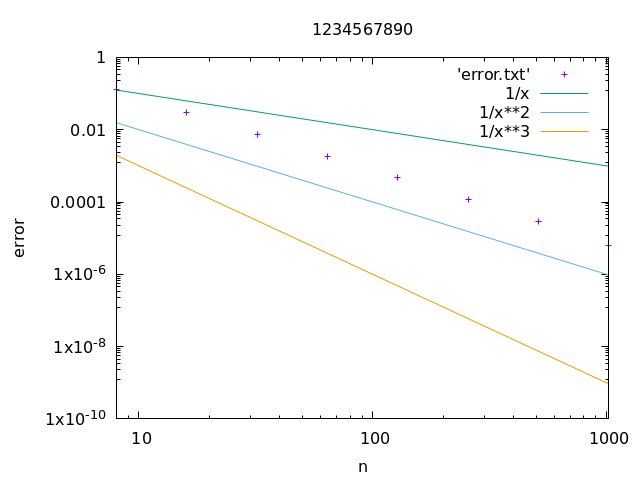
Modify the code to print the error e_n := |y_n - y(5)| for n = 2^m, m = 3, 4, \ldots 10, where y(5) = \exp(1 - \cos 5) is the exact value of the solution. Submit the code.
Plot the graph of e_n vs. n with logarithmic scale on both axes. In the same plot, plot also 1/n, 1/n^2 and 1/n^3. Submit the plot.
Exercise 2.
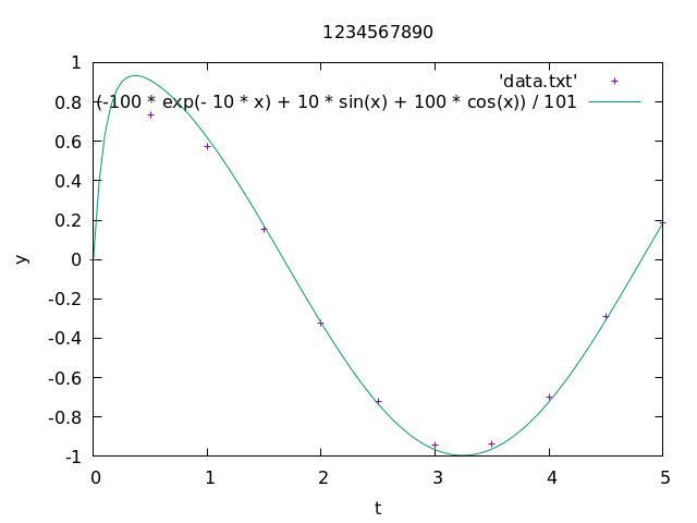
Implement the backward Euler method introduced above in Fortran to find the numerical solution of the ODE y' = -10(y - \cos t) with initial data y(0) = 0 on interval (0, 5).
Plot the numerical solution using gnuplot for n = 10 and the exact solution y(t) = \frac{-a^2\exp(-at) + a\sin(t) + a^2\cos(t)}{a^2 + 1}, with a = 10. Do not forget to add labels for each axis (x-axis has label
tand y-axis has labely). Submit the plot.Submit the Fortran code that you used to produce the numerical solution for 1.
Exercise 3.
Implement a Fortran program that uses the midpoint method to solve the system \begin{aligned} y_1' &= y_2\\ y_2' &= -y_1 \end{aligned} with initial data y_0 = (1, 0) on interval (0, 10).
Plot the numerical solution using gnuplot for n = 20 with values y_1 on the horizontal axis and values y_2 on the vertical axis. Submit the plot.
Submit the Fortran code you used to produce data in 1.
- Submit the plot of the graph of the error e_n = \|y_n - y(10)\| for n = 2^m, m = 3, 4, \ldots, 10. Here y(10) = (\cos 10, -\sin 10) is the exact solution and \|p\| = \sqrt{p_1^2 + p_2^2} is the Euclidean norm of an {\mathbb{R}}^2 vector. Plot 1/n, 1/n^2 and 1/n^3 in the same plot to be able to verify that it is a second-order method.
Exercise 4.
Implement a Fortran program that uses the backward Euler method to solve the system \begin{aligned} y_1' &= y_2\\ y_2' &= -y_1 \end{aligned} with initial data y_0 = (1, 0).
Plot the solution with n = 100 on interval (0, 10) (time step h = 10 / 100) in the y_1, y_2 plane as in the previous exercise. Submit the plot.
Submit the Fortran code you used to produce data in 1.
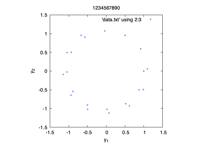
This is how some of the plots are expected to look like:
1-1
1-3
2-1
3-1
